Hidden Markov Models
We're going to move on from the Box-Jenkins and frequency domain approaches to our data to some more exciting and novel approaches. We're not done with them, and will likely return to these approaches in later posts, particularly as we focus on automation of analysis in more detail.
One of the challenges of prior approaches to time series analysis is that many of these techniques are based on the series being a normal (Gaussian) distributed, continuous variable. The reasons for why other nonlinear distributions come up short are somewhat complex, but can generally be summed up as due to the fact that for groups of a Gaussian variable, the average of the pooled sample is the same as the average of each group's average. For a nonlinearly distributed variable, the overall average is not necessarily the same as the average of each group. (This is the reason that analysis on nonlinear panel data requires one or the other of two different methods--marginal models obtained from general estimating equations and mixed effects models--depending on the goal. Marginal models are used for population average inference, while mixed effects models are used for individual prediction). For time series data, where there are generally many observations on a single individual over time (as opposed to most longitudinal approaches based on a couple of repeated measures per person), either of these methods are impractical due to the size of the covariance matrix needed to be estimated and large number of parameters. For that reason, alternative approaches were needed to analyze a time series of non-Gaussian data; one of which is called the Hidden Markov Model.
The Hidden Markov Model
The following description is based on the very excellent textbook about Hidden Markov Models by Zucchini and colleagues called Hidden Markov Models for Time Series: An Introduction Using R, Second Edition (CRC Press, 2016). I would highly recommend this book for anyone interested in performing time series analysis with HMM, and it also contains some great R code templates, which we'll be referencing throughout this post.
Mixture Distributions
An understanding of Hidden Markov Models (HMM) starts with the concept of a mixture model. A mixture model is basically a variable whose distribution can be described as a mixture of distributions with different parameters. For example, in Figure 1, we see a variable that displays a non-normal distribution, with three apparent peaks that reflect a mixture of three normal distributions. It's not important for our purposes, but this is an independent distribution, in which the values are distributed IID (independent and identically distributed).
The mixture distribution in Figure 1 is composed of three unobserved states, or components (C), in which the value observed is a function of the underlying probability of the state. In this case, for C = 1, Pr(x) ~ N(μ = 5, σ); for C = 2, Pr(x) ~ N(μ = 10, σ); and for C = 3, Pr(x) ~ N(μ = 15, σ). The probability of being in a given state is determined by a probability δ1 for C = 1; δ2 for C = 2; and δ3 (= 1 - (δ1 + δ2)) for C = 3. In Figure 1, the mixture is composed of three normal distributions, but it can be a mixture of any number of different distributions (e.g., two state with poisson and normal distributions mixed). The process of fitting mixture models is typically via maximum likelihood, although often parameters must be transformed prior to fitting, as we'll see in our code later.
Figure 1. Mixture distribution of three normal distributions with means of 5, 10, and 15. See text for details. From Wikipedia.org.
Markov Chains
A discrete-time Markov chain is a set of random variables C for which the probability of the next value in the chain is only conditional on the most recent value:
Pr(Ct+1 | Ct,...,C1) = Pr(Ct+1 | Ct)
This is known as the Markov property, and it is important for time series because it allows us to relax the assumption of independence seen above for indepedent mixture models, which as we know is critical for time series analysis since the values often display autocorrelation.
The probability of transitioning states in a Markov chain (moving from C1 to C2 is called the transition probability. If the probability is independent of a given point in time, then the Markov chain is called homogenous, and if the probability of a given state at a given time (i.e., δ1, δ2, and δ3 are stable), then we call the Markov chain stationary. In addition, a stationary Markov chain must be homogenous, irreducible, and aperiodic. We will see below that models can be constructed for both stationary and non-stationary Markov chains, the latter case requiring us to provide an estimate of the initial distribution of state probabilities (δ).
Hidden Markov Model
At this point you can probably start to see how we might combine the concept of mixture models/distributions, which allow us to model complex non-Gaussian distributions, and Markov models, which allow a mechanism to account for the lack of independence of random variables over time. A hidden Markov model (HMM) is basically a combination of these two, through combination of two processes: Parameter process and a State-dependent process.
The state-dependent process is basically the process of determining the probability of observing a given value (X) at a point in time (t) given a particular state distribution (C) active at that time: Pr(Xt | Ct). The parameter-dependent process is the process for determining a given state distribution (Ct) given the prior state distribution (Ct-1), which as we saw above is the only determinant of a given state for a first-order Markov chain: Pr(Ct | Ct-1).
In discrete HMMs, there are a pre-determined number of states (C1, C2,..., Cm), and the probability of a given state at a given time is (δ1, δ2,..., δm). The transition probability matrix (Γ) determines how the distribution of δ changes over time. Figure 2 below displays how at each point in time (1-4) the X value observed is based on the probability distribution C at that time. The parameters of the probability distribution (or the type of distribution) are different for different states. We won't delve into the estimation process, or other more complicated topics like non-discrete HMMs, hidden semi-Markov models, or HMM with random variables on this post, but there are excellent descriptions and examples provided for these topics in Zucchini et al.
Figure 2. Hidden Markov Model with observations (X) generated from distributions (C), with transition probability matrix (Γ). See text for details.
Hidden Markov Model in Action
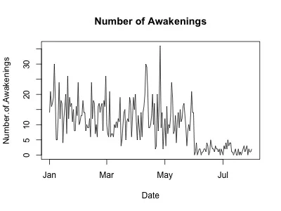
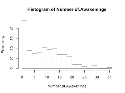
The following example is a basic HMM performed on my Fitbit data using code adapted from Zucchini et al. The data we'll be analyzing is for the number of times awakened at night as recorded by my Fitbit device, which as you can see from the histogram and time series (Figure 3), is not normally distributed. The code is available for download on our Github page.
Figure 3. Time series (left) and histogram (right) of number of awakenings as recorded by my Fitbit device. See text for details.
Selecting a model
Since we have no good reason for suspecting a given number of states ahead of time, we'll plan to run models using 2, 3, and 4 states, with both assumption of stationary Markov chains and nonstationary chains. Since the data we'll be examining are measuring counts, we'll plan to use Poisson distributions to describe the data. The nice thing about a Poisson distribution is that it only requires one parameter (λ), which is both the mean and variance. Although we haven't tested it formally, we suspect that the variance of our data is greater than λ, a situation referred to as overdispersion. There are other methods for managing overdispersion, for example using other families of distribution (e.g., negative binomial) in a general linear model, but one nice method for managing overdispersion is use of HMM.
Below are the AIC and BIC for each type of model. As we can see, the model with the lowest for both is a 3-state stationary model.
2-state Stationary: AIC 1289.3, BIC 1302.7
2-state Nonstationary: AIC 1290.4, BIC 1307.2
3-state Stationary: AIC 1196.1, BIC 1226.3
3-state Nonstationary: AIC 1197.7, BIC 1234.6
4-state Stationary: AIC 1202.5, BIC 1256.1
4-state Nonstationary: AIC 1205.6, BIC 1269.3
The 3-state stationary model has the following parameters. The mean (λ) for state 1 is 1.7, state 2 is 8.8, and state 3 is 17.7. In other words, while the HMM is in each of those states, the number of awakenings on a given night is a function of a Poisson process with mean of λ. The stationary probability distribution of each state over time (δ) is 0.35 for state 1, 0.34 for state 2, and 0.31 for state 3. The transition probability matrix is below:
State 1 State 2 State 3
State 1 0.99 0.00 0.01
State 2 0.00 0.67 0.33
State 3 0.02 0.36 0.62
As we can see, there's little transitioning out of state 1, and state 2 and 3 spend about 2/3 of the time in the same state and about 1/3 transitioning to the other. Using a process called decoding, we can plot the most likely state at any given point in time along with our time series data (Figure 4). This can be done using either local decoding, or an algorithm called the Viterbi algorithm for global decoding. The Github code uses both, but since the plots are virtually identical, we only show the local decoding.
Figure 4. Local decoding of three-state HMM. See text for details.
The decoding plot demonstrates why a three-state model would fit the data well. There's clearly a separate process happening early in the year, with a rapid decline in number of awakenings in the summer. Is this because it's more relaxing in summer and thus I was disturbed from sleep less often? Or is it (more likely) reflective of a technical issue with the sleep monitor (or sleep monitor algorithm) on my Fitbit device? Certainly if we were able to collect data for a longer period of time, we could examine possible seasonal patterns.
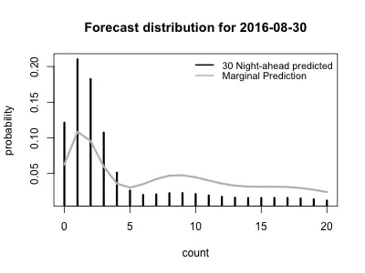
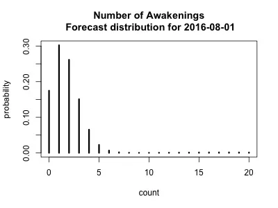
Although in this case it's probably less informative, we can use our HMM to forecast the expected number of awakenings for both the following night (One night ahead, Figure 5, left) and for 30 nights ahead (Figure 5, right). The latter plot shows both the marginal forecast (think of this as the long-term forecast) and one generating from running our (hidden) Markov chain the next 30 nights separately. As expected, we're dominated by state 1 and thus the expected number of awakenings is going to be low. Because it also includes the marginal prediction from all of the prior data, Figure 5 (right) shows two different levels of probability. The forecast based on the most recent values (the 30-night ahead prediction) places higher probability on a lower number of nightly awakenings. In contrast, the marginal prediction is more diffuse, since it places greater 'weight' on the number of awakenings earlier in the dataset. Which is correct? Tough to know since we don't know for sure what the underlying process is that is responsible for each of the three states.
Figure 5. Left, forecast for the probability of a given number of awakenings for the next day following data collection (8/1/2016, data collection ended on 7/31/2016). Right, the 30-night ahead prediction and marginal prediction forecasts for 30 days ahead (8/30/2016). See text for details.
Hidden Markov models are not only a great method for handling discrete time series data, they can help provide some insight into the data generating process. They are widely used for everything from earthquake prediction (the example used in the Zucchini book) to speech recognition, and we will come back to them often for analysis of time series data.


