States and HMMs
In the last post, we introduced the hidden Markov model as a powerful tool to explore the potential generating processes behind our data. In this post, we'll delve a bit more into the different uses and interpretations of HMM applied to monitor data.
It is worth pointing out at this point that the monitor data we are working with has already been processed to make the inferences about what activity we are performing at the time that the monitor's accelerometer (or other sensors) are examining the data. For an example of how HMM are applied to the raw accelerometer data to make determinations about the type of activity being performed, check out a great paper in Plos One by Witowski and colleagues. At that level, the monitor is trying to translate the impulse counts generated by three dimensional movement of the accelerometer into types of activity (exercise, sedentary, sleep). As the authors point out, hidden Markov models provide an excellent method to model these types of activity. Whether this is the approach Fitbit or other activity monitors use is unknown given the proprietary nature of these companies, and unknown to us generally. However, we may keep these concepts in mind as we apply these methods to data where we are in fact working with the raw data. We should also bear in mind that Fitbit (or another company) may change up their algorithms at any time, which has the potential to lead us to draw false inferences with our data. We saw this in the prior post and in Figure 1 below, where the number of awakenings on my Fitbit dropped from an average of around 8-15 per night to around 1-2 per night after a certain day. I can guarantee that this was not a change in my actual awakenings, and that in all likelihood this change reflected the application of a more accurate algorithm by Fitbit to their data (waking from sleep a few times a night is a lot more likely that waking over 30 times in a night).
Figure 1. Three-state HMM applied to number of awakenings from my Fitbit monitor. See prior post for details.
Technical outliers aside, the latent information that we are most interested in from these models is what underlying process is driving the behavior being collected by the monitor. For example, is the amount of exercise on a given day a reflection of my state of wellness on that particular day? Is it a reflection of the amount of free time available on that day? Or is it just part of a cyclical pattern that we might have uncovered with approaches described previously that would be recreated using HMMs. To tease these ideas apart, let's take a look at a couple of the variables obtained from my Fitbit.
Models for Steps
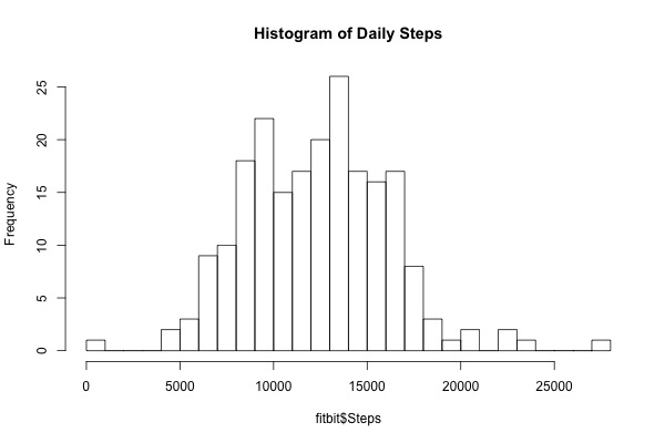
As shown in the histogram in Figure 2 below, the number of steps per day is pretty evenly distributed, although not completely normal. There appear to be at least two separate peaks in the number of daily steps, which suggests that there are some days when I may be in a more 'active' state and others when I'm less active. An HMM would be perfect to try to uncover these states.
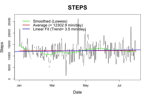
Figure 2. Left, time series of number of daily steps, with average, linear trend, and smoothed. Right, histogram of number of daily steps.
Using an R package called depmixS4, we can develop HMM using Gaussian distributions for our step data. We'll plan to fit this data using up to 4 states, and examine the AIC and BIC to choose the best model based on fit and parsimony.
States AIC BIC
1 4082.2 4088.9
2 4095.7 4109.2
3 4066.8 4113.7
4 4076.2 4153.3
As we can see above, based on the BIC, the best model is the one state model, which is basically a simple regression model without states. Based on the AIC, the three state model is the best one. And based on our simple idea of 'healthy' and 'non-healthy' days, the two state model is appropriate. To explore the latter two models, let's examine the predicted distribution parameters and transition probability matrices (TPM).
For a model with 2 states, the observed data are generated from two Gaussian distributions, with states as below:
Mean SD
State 1: 12091 3507
State 2: 23252 2557
The transition probability matrix (TPM) for this model is below:
State 1 State 2
State 1 0.98 0.02
State 2 0.90 0.10
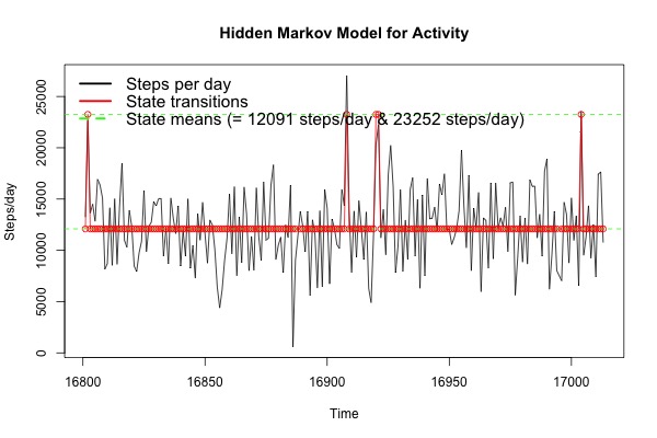
Based on this model, I spend most of my time in state 1, which has a mean of about 12k steps/day, with occasional episodes where I transition up to state 2, with a mean of 23k steps/day. Perhaps this is because some days I feel really active, and most days I'm only somewhat active. However, as we see in the graph below (and can infer from the TPM above), it is pretty rare that I spend much time in the 'very active' state.
Figure 3. 2-State HMM for Daily Steps. See text for details.
The information for 3-state model is below:
Distribution parameters: TPM:
Mean SD State 1 State 2 State 3
State 1 9274.9 1673.6 State 1 0.05 0.95 0.00
State 2 14210.4 1860.2 State 2 0.48 0.17 0.34
State 3 12816.7 5133.2 State 3 0.32 0.13 0.56
Noteworthy is that state 3 is a lower mean than state 2, which is likely because of the order these occur in the model. As noted from the TPM and the global decoding graph below, there is much more movement between these different states in this model than in the 2 state model.
Figure 4. 3-state HMM for Daily Steps. See text for details.
Binary Outcome HMM
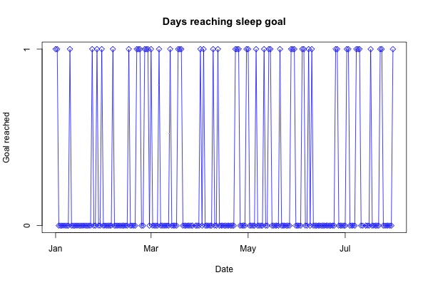
An interesting potential use of HMMs is modeling binary outcomes, such as on/off or yes/no events, with the notion that latent variables might imply some degree of 'health' or 'wellness' during which susceptibility to a given disease is greater or less. Since Fitbit doesn't itself track these types of things, I've created a variable called 'sleepGoal' to indicate whether the number of minutes slept in a night is greater than 480 (8 hours). Figure 5 below displays how often over the course of time I reached that sleep goal.
Figure 5. Binary time series for sleep goal (0, 1). See text for details.
As we can see from the figure, I only met the sleep goal about 25% of the time (need to work on that...). One of the challenges of time series analysis is that many of the methods are based on Gaussian distributions. Autocorrelation between discrete outcomes is much more challenging to model, which is another reason why HMM is such a powerful tool in time series analysis.
Like above with the Gaussian variable distributions, we'll use the 'depmixS4' package in R to fit HMM for our series; in this case, the family we'll use will be the binomial family, with the logit link function. We'll fit a model without any states (an intercept-only logit model), and up to 4 state models. The resulting AIC and BIC are below:
States AIC BIC
1 237.6 241.0
2 245.5 262.3
3 242.2 279.1
4 255.5 319.1
Unfortunately for our HMMs, none of the models are better than a single state model. However, for illustration purposes, we'll examine the 2-state model since it had the lowest BIC, and also fits better with our two-state latent idea of good and bad days.
The probability parameter of the binomial distribution (π) is given below:
Parameters: TPM:
Pi State 1 State 2
State 1 0.22 State 1 0.49 0.51
State 2 0.28 State 2 0.71 0.29
Figure 6 (below) shows the decoded time series with these two states. We see that these two states fluctuate around the overall average probability (0.25) of reaching the goal sleep on a given night. (Note, as is evident with running the R script on Github, the function did not converge for the 2-state model. We are using parameters estimated at the maximum allowable iteration, but be aware that these estimates are probably not at the global maximum. We proceed regardless with discussion purely for illustration purposes). The information from this model is not particularly informative, and since it appears that we spend roughly equal amounts of time between the two states, which themselves are not particularly different in terms of probability of reaching my sleep goal, not much additional information appears to be evident about my sleep patterns.
Figure 6. HMM decoded plot for sleep goal. See text for details.
Zero-inflated HMM
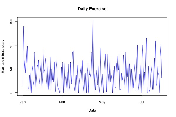
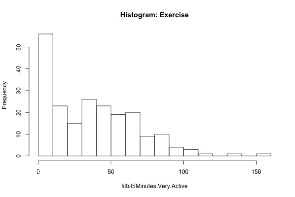
In a last illustration, we'll examine the fairly common situation with this type of data in which we have a zero-inflated dataset. For an example of such a dataset, we will use the 'exercise' designation of my Fitbit called Minutes.Very.Active. As you can see from the graphs below in Figure 7, the data has a high amount of zero-inflation.
Figure 7. Left, Time series of minutes of daily exercise. Right, histogram of daily minutes of exercise. See text for details.
To examine zero-inflated HMM, we'll use a special package in R (developed by Zekun Xu) called ziphsmm. This package, which can fit HMM and a more generalized version called hidden semi-Markov models (we'll probably cross these as well at a later date), allows us to fit an HMM with Poisson distributions and allows for one of the states to have a zero-inflated proportion (which we designate with our function call (see Github code for details).
Fitting zero-inflated HMM with Poisson distribution for up to 5 states, we get the following results:
AIC BIC
2-State 2648.0 2668.1
3-State 2157.8 2198.1
4-State 2063.9 2131.0
5-State 2000.9 2101.4
In this case, it appears that the more states we include, the better the fit for both AIC and BIC. Ideally we would continue to increase until there was some inflection point in these measures, although since this is simply for exploratory purposes, we'll stop here. For the 5 state model, the mean and TPM are as follows:
Means: TPM:
State1: 6.4 min/day State_1 State_2 State_3 State_4 State_5
State2: 21.5 min/day State 1 0.13 0.10 0.48 0.22 0.08
State3: 45.8 min/day State 2 0.13 0.23 0.23 0.30 0.11
State4: 67.7 min/day State 3 0.21 0.24 0.24 0.17 0.15
State5: 102.6 min/day State 4 0.21 0.36 0.18 0.05 0.19
State 5 0.16 0.21 0.25 0.19 0.20
Proportion zero: 0.43
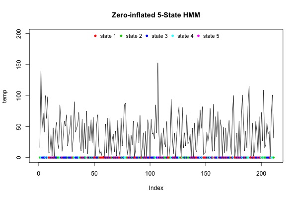
This function also includes a nice built-in decoding and graph function, which outputs the graph below in Figure 8.
Figure 8. Zero-inflated 5-state Poisson HMM, decoded with Viterbi algorithm. See text for details.
From a qualitative viewpoint, we can see that there appear to be more blue dots in Figure 8 than other colors, which is what we would expect based on the TPM above, in which the values for transitions to State 3 are the highest. The overall average minutes of exercise for this dataset is 37.6 min/day, which is between states 2 and 3. That none of the states are at the average suggests that there is no 'average day' for exercise, and the single-state Poisson model (not zero-inflated) provides an AIC of 6785.9 and BIC of 6789.3, both of which are well above the estimates above (although the BIC was calculated using a different approach). As such, our 5-state zero-inflated model is an improvement over a simple Poisson model, although we are left to determine what the meaning is for the 5 latent states. The order of dots at the bottom of Figure 8 does not appear to follow any particular cyclical pattern, and so we are at a loss to explain what might account for 5 (and probably more) states of exercise daily.
So that's some more examples of hidden Markov models in action using my own Fitbit data. For all of the code, and primary dataset used, please see our Github page.


